2.3. Figure 3-variation - Net-zero CO2 emissions systems

Licensed under the MIT License.

This notebook is part of a repository to generate figures and analysis for the manuscript

Keywan Riahi, Christoph Bertram, Daniel Huppmann, et al.  Cost and attainability of meeting stringent climate targets without overshoot Nature Climate Change, 2021 doi: 10.1038/s41558-021-01215-2

The scenario data used in this analysis should be cited as

ENGAGE Global Scenarios (Version 2.0) doi: 10.5281/zenodo.5553976

The data can be accessed and downloaded via the ENGAGE Scenario Explorer at https://data.ece.iiasa.ac.at/engage. Please refer to thelicenseof the scenario ensemble before redistributing this data or adapted material.

The source code of this notebook is available on GitHub at https://github.com/iiasa/ENGAGE-netzero-analysis. A rendered version can be seen at https://data.ece.iiasa.ac.at/engage-netzero-analysis.

from pathlib import Path
import numpy as np
import pandas as pd
import matplotlib.pyplot as plt

import pyam

from utils import get_netzero_data

Import the scenario snapshot used for this analysis and the plotting configuration

data_folder = Path("../data/")

output_folder = Path("output")
output_format = "png"
plot_args = dict(facecolor="white", dpi=300)

rc = pyam.run_control()
rc.update("plotting_config.yaml")

df = pyam.IamDataFrame(data_folder / "ENGAGE_fig3.xlsx")

pyam - INFO: Running in a notebook, setting up a basic logging at level INFO
pyam.core - INFO: Reading file ../data/ENGAGE_fig3.xlsx
pyam.core - INFO: Reading meta indicators

All figures in this notebook use the same scenario.

scenario = "EN_NPi2020_1000"

Apply renaming for nicer plots.

df.rename(model=rc['rename_mapping']['model'], inplace=True)
df.rename(region=rc['rename_mapping']['region'], inplace=True)

The REMIND model does not reach net-zero CO2 emissions before the end of the century in the selected scenario used in these figures.

It is therefore excluded from this notebook.

df = (
    df.filter(scenario=scenario)
    .filter(model="REMIND*", keep=False)
    .convert_unit("Mt CO2/yr", "Gt CO2/yr")
)

Prepare CO2 emissions data

Aggregate two categories of “Other” emissions to show as one category.

components = [f"Emissions|CO2|{i}" for i in ["Other", "Energy|Demand|Other"]]
df_other = df.aggregate(variable="Emissions|CO2|Other", components=components)
df = df.filter(variable=components, keep=False).append(df_other)

sectors_mapping = {
    "AFOLU": "AFOLU",
    "Energy|Demand": "Energy Demand",
    "Energy|Demand|Industry": "Industry",
    "Energy|Demand|Transportation": "Transportation",
    "Energy|Demand|Residential and Commercial": "Buildings",
    "Energy|Supply": "Energy Supply",
    "Industrial Processes": "Industrial Processes",
    "Other": "Other"
}

# explode short dictionary-keys to full variable string
for key in list(sectors_mapping):
    sectors_mapping[f"Emissions|CO2|{key}"] = sectors_mapping.pop(key)

df.rename(variable=sectors_mapping, inplace=True)
sectors = list(sectors_mapping.values())

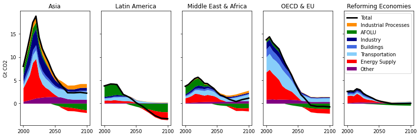
Development of emissions by sector & regions in one illustrative model

This section generates Figure 1.1-15 in the Supplementary Information.

model='MESSAGEix-GLOBIOM'

df_sector = (
    df.filter(variable=sectors)
    .filter(region='World', keep=False)
    .filter(variable='Energy Demand', keep=False)  # show disaggregation of demand sectors
)

_df_sector = df_sector.filter(model=model)
fig, ax = plt.subplots(1, len(_df_sector.region), figsize=(12, 4), sharey=True)

for i, r in enumerate(_df_sector.region):
    (
        _df_sector.filter(region=r)
        .plot.stack(ax=ax[i], total=dict(lw=3, color='black'), title=None, legend=False)
    )

    ax[i].set_xlabel(None)
    ax[i].set_ylabel(None)
    ax[i].set_title(r)

plt.tight_layout()
ax[0].set_ylabel("Gt CO2")
ax[i].legend(loc=1)

plt.tight_layout()
fig.savefig(output_folder / f"fig3_annex_sectoral_regional_illustrative.{output_format}", **plot_args)

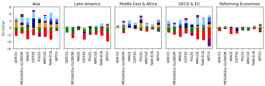
Emissions by sectors & regions in the year of net-zero

This section generates Figure 1.1-16 in the Supplementary Information.

lst = []

df_sector.filter(region="Other", keep=False, inplace=True)

df_netzero = get_netzero_data(df_sector, "netzero|CO2", default_year=2100)

fig, ax = plt.subplots(1, len(df_sector.region), figsize=(12, 4), sharey=True)

for i, r in enumerate(df_sector.region):
    df_netzero.filter(region=r).plot.bar(ax=ax[i], x="model", stacked=True, legend=False)
    ax[i].axhline(0, color="black", linewidth=0.5)

    ax[i].set_title(r)
    ax[i].set_xlabel(None)

ax[i].set_ylim(-6, 6)

plt.tight_layout()
fig.savefig(output_folder / f"fig3_annex_sectoral_regional_netzero.{output_format}", **plot_args)