2.3. Figure 3 - Net-zero CO2 emissions systems

Licensed under the MIT License.

This notebook is part of a repository to generate figures and analysis for the manuscript

Keywan Riahi, Christoph Bertram, Daniel Huppmann, et al.  Cost and attainability of meeting stringent climate targets without overshoot Nature Climate Change, 2021 doi: 10.1038/s41558-021-01215-2

The scenario data used in this analysis should be cited as

ENGAGE Global Scenarios (Version 2.0) doi: 10.5281/zenodo.5553976

The data can be accessed and downloaded via the ENGAGE Scenario Explorer at https://data.ece.iiasa.ac.at/engage. Please refer to thelicenseof the scenario ensemble before redistributing this data or adapted material.

The source code of this notebook is available on GitHub at https://github.com/iiasa/ENGAGE-netzero-analysis. A rendered version can be seen at https://data.ece.iiasa.ac.at/engage-netzero-analysis.

from pathlib import Path
import numpy as np
import pandas as pd
import matplotlib.pyplot as plt
import seaborn as sns

import pyam

from utils import get_netzero_data

Import the scenario snapshot used for this analysis and the plotting configuration

data_folder = Path("../data/")

output_folder = Path("output")
output_format = "png"
plot_args = dict(facecolor="white", dpi=300)

rc = pyam.run_control()
rc.update("plotting_config.yaml")

df = pyam.IamDataFrame(data_folder / "ENGAGE_fig3.xlsx")

pyam - INFO: Running in a notebook, setting up a basic logging at level INFO
pyam.core - INFO: Reading file ../data/ENGAGE_fig3.xlsx
pyam.core - INFO: Reading meta indicators

Panels a, b, d and e in this figure use the same scenario.

scenario = "EN_NPi2020_1000"

Apply renaming for nicer plots.

df.rename(model=rc["rename_mapping"]["model"], inplace=True)
df.rename(region=rc["rename_mapping"]["region"], inplace=True)

model_format_mapping = {
    "MESSAGEix-GLOBIOM": "MESSAGEix-\nGLOBIOM",
}

def format_model_name(i, model_format_mapping):
    name = i.get_text()
    for key, value in model_format_mapping.items():
        name = name.replace(key, value)

    return name

Prepare CO2 emissions data

Aggregate two categories of “Other” emissions to show as one category.

components = [f"Emissions|CO2|{i}" for i in ["Other", "Energy|Demand|Other"]]
df_other = df.aggregate(variable="Emissions|CO2|Other", components=components)
df = df.filter(variable=components, keep=False).append(df_other)

sectors_mapping = {
    "AFOLU": "AFOLU",
    "Energy|Demand": "Energy Demand",
    "Energy|Demand|Industry": "Industry",
    "Energy|Demand|Transportation": "Transportation",
    "Energy|Demand|Residential and Commercial": "Buildings",
    "Energy|Supply": "Energy Supply",
    "Industrial Processes": "Industrial Processes",
    "Other": "Other"
}

# explode short dictionary-keys to full variable string
for key in list(sectors_mapping):
    sectors_mapping[f"Emissions|CO2|{key}"] = sectors_mapping.pop(key)

df.rename(variable=sectors_mapping, inplace=True)
sectors = list(sectors_mapping.values())

The REMIND model does not reach net-zero CO2 emissions before the end of the century in the selected scenario used in Panels a, b, d and e.

It is therefore excluded from this notebook.

df_sector = (
    df.filter(region="World", scenario=scenario, variable=sectors)
    .filter(variable="Energy Demand", keep=False)  # show disaggregation of demand sectors
    .filter(model="REMIND*", keep=False)
    .convert_unit("Mt CO2/yr", "Gt CO2/yr")
)

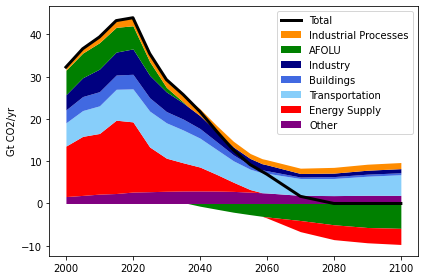
Panel a - Development of emissions by sector in one illustrative model

model="MESSAGEix-GLOBIOM"

fig, ax = plt.subplots(figsize=(6, 4))

(
    df_sector.filter(model=model)
    .plot.stack(ax=ax, title=None, total=dict(lw=3, color="black"))
)

ax.set_xlabel(None)
plt.legend(loc=1)

plt.tight_layout()
fig.savefig(output_folder / f"fig3a_sectoral.{output_format}", **plot_args)

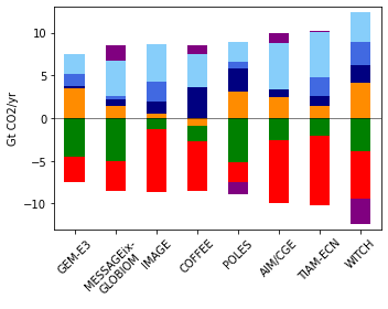
Panel b - Emissions by sector in the year of net-zero

The function get_netzero_data is defined in the file utils.py in this folder.

df_netzero_sector = get_netzero_data(df_sector, "netzero|CO2", default_year=2100)

fig, ax = plt.subplots(figsize=(5, 4))

df_netzero_sector.plot.bar(ax=ax, x="model", title=None, stacked=True, legend=False)
ax.axhline(0, color="black", linewidth=0.5)

plt.xlabel(None)
ax.set_xticklabels([format_model_name(i, model_format_mapping) for i in ax.get_xticklabels()])

plt.xticks(rotation=45)
ax.set_ylim(-13, 13)

plt.tight_layout()
fig.savefig(output_folder / f"fig3b_sectoral_year_netzero.{output_format}", **plot_args)

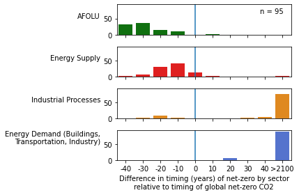
Panel c - Timing of net-zero CO2 emissions for different sectors

The timing of net-zero for different sectors relative to the timing of net-zero global total CO2 (blue line at zero). The histograms include all pathways that limit temperature to <2 °C.

budget_groups = [600, 900, 1200]

def budget_classification(x):
    for b in budget_groups:
        if x < b:
            return f"below {b} Gt"
    return np.nan

df.set_meta(meta=df.meta["cumulative_emissions_2100"].apply(budget_classification),
            name="budget_range")

def _cross_threshold(x):
    y = pyam.cross_threshold(x, threshold=10)  # the unit is Mt CO2
    return y[0] if len(y) else np.inf

def calculate_netzero(_df):
    cross = _df.apply(_cross_threshold, raw=False, axis=1)
    cross.index = cross.index.droplevel(["region", "variable", "unit"])
    return cross

cols = ["category", "category_peak", "budget_type", "budget_range", "scenario_family", "cumulative_emissions_2100"]

df_sector_nz = df.filter(region="World", variable=sectors, category_peak=["1.5C (with low overshoot)", "2C"])

netzero_sector = df_sector_nz.meta[cols]

for v in sectors:
    _co2 = df_sector_nz.filter(variable=v).timeseries()
    netzero_sector[v] = calculate_netzero(_co2) - df_sector_nz.meta["netzero|CO2"]

x = netzero_sector.set_index(cols, append=True).stack().reset_index().rename(columns={0: "value", "level_8": "sector"})

/var/folders/5h/q1v5dh_d1gx94zmd0rlvysgh0000gn/T/ipykernel_3098/966498754.py:3: SettingWithCopyWarning:
A value is trying to be set on a copy of a slice from a DataFrame.
Try using .loc[row_indexer,col_indexer] = value instead

See the caveats in the documentation: https://pandas.pydata.org/pandas-docs/stable/user_guide/indexing.html#returning-a-view-versus-a-copy
  netzero_sector[v] = calculate_netzero(_co2) - df_sector_nz.meta["netzero|CO2"]

netzero_bins = [-40, -30, -20, -10, 0, 10, 20, 30, 40, ">2100"]

def assign_nz_bin(x):
    for b in netzero_bins:
        try:
            if x < b:
                return b
        # this approach works as long as only the last item is a string
        except TypeError:
            return b

x["netzero"] = x.value.apply(assign_nz_bin)

is_inf = [np.isinf(v) for v in x.value]
not_inf = np.logical_not(is_inf)

_max = max(x.loc[not_inf, "value"])

x["value_"] = x.value
x.loc[is_inf, "value_"] = _max + 10

The pyam package does not support histogram-type plots, so panel d is implemented directly in seaborn.

sector_list = ["AFOLU", "Energy Supply", "Industrial Processes", "Energy Demand"]

n = len(sector_list)

fig, ax = plt.subplots(n, 1, figsize=(6, 4), sharex=True, sharey=True)

_x = x[[i in ["1.5C (with low overshoot)", "2C"] for i in x.category_peak]]
_x = _x[_x.scenario_family == "NPi"]

for i, s in enumerate(sector_list):
    sns.countplot(ax=ax[i], data=_x[_x.sector == s], x="netzero", order=netzero_bins,
                  color=rc["color"]["variable"][s])
    ax[i].set_xlabel(None)
    ax[i].set_ylabel(s, rotation=0, horizontalalignment="right")
    ax[i].axvline(x=4)

ax[3].set_ylabel("Energy Demand (Buildings,\nTransportation, Industry)",
                 rotation=0, horizontalalignment="right")
ax[3].set_xlabel("Difference in timing (years) of net-zero by sector\nrelative to timing of global net-zero CO2",)

pyam.plotting.set_panel_label(f"n = {len(_x[_x.sector == s])}", ax=ax[0], x=0.82, y=0.7)

plt.tight_layout()
fig.savefig(output_folder / f"fig3c_sectoral_range_netzero.{output_format}", **plot_args)

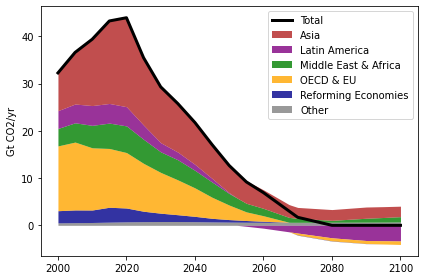
Panel d - Development of emissions by region in one illustrative model

df_regional = (
    df.filter(region="World", keep=False)
    .filter(scenario=scenario, variable="Emissions|CO2")
    .filter(model="REMIND*", keep=False)
    .convert_unit("Mt CO2/yr", "Gt CO2/yr")
)

fig, ax = plt.subplots(figsize=(6, 4))

(
    pyam.IamDataFrame(
        df_regional.filter(model=model)
        .timeseries()
        .fillna(0)
     ).plot.stack(ax=ax, stack="region", title=None, alpha=0.8, total=dict(lw=3))
)

plt.legend(loc=1)
ax.set_xlabel(None)

plt.tight_layout()
fig.savefig(output_folder / f"fig3d_regional.{output_format}", **plot_args)

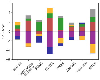
Panel e - Emissions by region in the year of net-zero

The function get_netzero_data is defined in the file utils.py in this folder.

df_netzero_regional = get_netzero_data(df_regional, "netzero|CO2", default_year=2100)

fig, ax = plt.subplots(figsize=(5, 4))

df_netzero_regional.plot.bar(ax=ax, x="model", bars="region", stacked=True, alpha=0.8, title=None, legend=False)

ax.axhline(0, color="black", linewidth=0.5)
ax.set_ylim(-6, 6)
ax.set_xticklabels([format_model_name(i, model_format_mapping) for i in ax.get_xticklabels()])
plt.xlabel(None)

plt.xticks(rotation=45)

plt.tight_layout()
fig.savefig(output_folder / f"fig3e_regional_year_netzero.{output_format}", **plot_args)

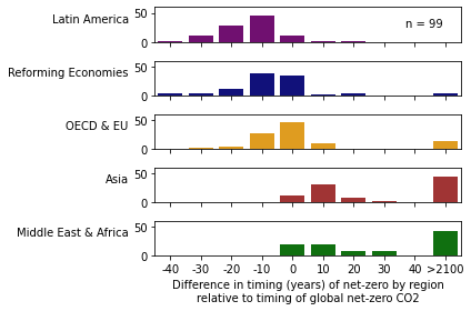
Panel f - Timing of net-zero CO2 emissions for different regions

The timing of net-zero for different regions relative to the timing of net-zero global total CO2 (blue line at zero). The histograms include all pathways that limit temperature to <2 °C.

cols = ["category", "budget_type", "budget_range", "scenario_family", "cumulative_emissions_2100"]

df_region_nz = (
    df.filter(region="World", keep=False).filter(variable="Emissions|CO2")
)

netzero_region = df_region_nz.meta[cols].copy()

for r in df_region_nz.region:
    if r == "Other":
        continue

    _co2 = df_region_nz.filter(region=r).timeseries()
    netzero_region[r] = calculate_netzero(_co2) - df_region_nz.meta["netzero|CO2"]

x = netzero_region.set_index(cols, append=True).stack().reset_index().rename(columns={0: "value", "level_7": "region"})

x["netzero"] = x.value.apply(assign_nz_bin)

regions = ["Latin America", "Reforming Economies", "OECD & EU", "Asia", "Middle East & Africa"]

n = len(regions)

fig, ax = plt.subplots(n, 1, figsize=(6, 4), sharex=True, sharey=True)

_x = x[[i in ["1.5C (with low overshoot)", "2C"] for i in x.category]]
_x = _x[_x.scenario_family == "NPi"]

for i, r in enumerate(regions):
    sns.countplot(ax=ax[i], data=_x[_x.region == r], x="netzero", order=netzero_bins,
                  color=rc["color"]["region"][r])
    ax[i].set_xlabel(None)
    ax[i].set_ylabel(r, rotation=0, horizontalalignment="right")
    plt.tight_layout()

pyam.plotting.set_panel_label(f"n = {len(_x[_x.region == r])}", ax=ax[0], x=0.82, y=0.55)

ax[4].set_ylim(0, 60)
ax[4].set_xlabel("Difference in timing (years) of net-zero by region\nrelative to timing of global net-zero CO2")

plt.tight_layout()
fig.savefig(output_folder / f"fig3f_regional_range_netzero.{output_format}", **plot_args)